In media headlines, we often encounter striking figures such as “420 million hectares of forest have been lost since 1990,” “40% of the planet’s terrestrial areas are degraded,” or “we have lost one-third of our wetlands.”
So how can we state figures that refer to such vast areas with such confidence? The answer lies in one of the most powerful products of modern remote sensing technologies: land cover datasets.
What Does Land Cover Tell Us?
“Land” is not merely a surface on which we walk; it is a living system that determines water quality and flow, local and regional climate dynamics, and the distribution of biodiversity, while also supporting fundamental needs such as shelter and food production. Being able to answer the question “what is where?” in a regular and measurable way is critical not only for understanding the present, but also for monitoring change and managing the future.
Before moving further, it is useful to clarify two concepts that are often confused. Land cover maps describe what physically covers the Earth’s surface, such as forest, cropland, water, bare ground, or built-up areas. Land use maps, on the other hand, explain the purpose for which those areas are used, such as agricultural production, recreation, industry, or settlement planning. Although these two concepts may seem very close in everyday language, from a remote sensing perspective a small distinction can lead to major consequences: a satellite sensor first captures the “cover,” whereas “use” often requires additional context, administrative information, and interpretation.
At this point, the issue rests on two simple but powerful questions: Where are natural resources, and what condition are they in? How is this condition changing over time?
From Papyrus to Marble: Land Cover Mapping Before the Satellite Era
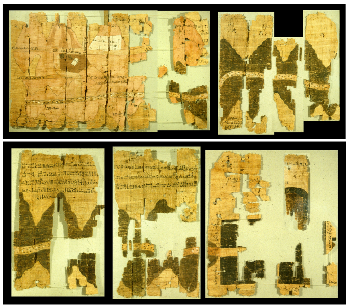
Global land cover datasets may appear to be products of the modern era, but the idea of recording resources and surface conditions is much older. One of the most striking starting points in this story is the Turin Papyrus Map, dated to around 1150 BCE. This map depicts a route through Wadi Hammamat in Egypt’s Eastern Desert; it marks resources such as gold mines and stone quarries as well as areas associated with an expedition, and it is regarded in the literature as one of the earliest examples of a geological map.4 The motivation behind it is surprisingly similar to that of today: Where is the resource, how can we reach it, and how should the activity be managed?
In the centuries that followed, this motivation became more systematic as it merged with state administration and taxation. In the Roman world, land surveying and cadastral records were critical tools for managing ownership and production. Although these records did not provide a “land cover raster” in the modern sense, they created a strong basis for reading the landscapes and land uses of particular periods.5
As time progressed, mining formed another branch of resource-oriented thematic documentation. In the 16th century, works that depicted mining sites, operational arrangements, and technical infrastructure through drawings began to answer the question “where is which resource, and how is it being exploited?” in a visual language. This approach intuitively foreshadowed today’s “layer” logic: resource, facility, transportation, settlement, and workforce were all parts of the same story.
By the 19th century, parcel-based mapping had become one of the most visible tools for systematically recording land. The tithe maps produced in England and Wales after 1836 numbered parcels and linked them with records, documenting categories such as fields, meadows, pastures, and woodlands. Their primary motivation was to make the taxation system more equitable and manageable.6 These maps are highly instructive for understanding how concrete and administratively driven the idea of “classification” was before the satellite era.
In all these examples, modern sensors did not exist; yet the question was the same. The difference is that we now have to answer this question not only locally, but globally and at regular intervals.
The Satellite Era: Speaking the Same Language at a Global Scale
The major turning point in the second half of the 20th century came with satellite systems capable of observing the Earth repeatedly. Early high-resolution imagery such as CORONA was not originally designed for scientific purposes; however, once its archives were declassified for civilian use, it offered an invaluable time window for retrospective land change studies.7
The major step that made this line of work operational was Landsat. Launched on 23 July 1972, ERTS-1, later renamed Landsat 1, is considered one of the first satellite programs designed for the systematic observation of natural resources. It mainstreamed the idea of producing comparable data for agriculture, forests, water, geology, and related fields.8
As satellite data matured, land cover maps evolved from purely academic products into infrastructures for public policy and planning. In Europe, the CORINE program, launched in 1985, became one of the symbolic examples of this transformation by aiming to produce a comparable land cover inventory at the continental scale.9 Similarly, national-scale products matured in different countries; in the United States, the NLCD (National Land Cover Database) approach is a good example of the institutionalization of Landsat-based classification and change monitoring.10
With the acceleration of global environmental change research in the 2000s, the need for global and regularly updated datasets became even more visible. MODIS-based annual land cover products represented one of the most prominent steps of this period by providing time-series inputs for climate models and ecosystem analyses.11 Later, open data policies, computational infrastructures, and the operational service logic of programs such as Copernicus created an ecosystem that made land cover maps more accessible and more up to date.12
Today, medium- to high-resolution Sentinel-2 observations, deep learning approaches, and global services have accelerated not only “map production” but also the detection of change. The main message of this article is this: global land cover datasets are not a technology showcase; they are a fundamental infrastructure for providing measurable answers to some of the world’s most essential environmental questions.
Why Have Global Land Cover Datasets Become So Numerous?
Today, we are not dealing with a single “global land cover map,” but with a multilayered data ecosystem produced for different purposes. The reason is clear: not every research question requires the same spatial detail, the same temporal coverage, or the same classification scheme. A 10 m Sentinel-2-based product may be meaningful for monitoring new urban development around a city, while coarser-resolution products with longer time series may be more useful for interpreting thirty-year global trends.
Therefore, global land cover datasets should not be evaluated by asking “which one is the best?” but rather by asking “which dataset is more appropriate for solving which problem?” High spatial resolution does not always mean more accurate results; similarly, an annually produced map does not always provide a reliable change analysis. The production algorithm, training data, class definitions, accuracy assessment, and sensor source of a dataset are at least as important as pixel size.
The 10 Meter Era: More Detailed, More Current, but Requiring More Careful Interpretation
One of the most notable transformations in global land cover mapping in recent years has been the spread of 10 m resolution products. Datasets such as ESA WorldCover, Dynamic World, ESRI 10m Land Use/Land Cover, and FROM-GLC10 have begun to provide more detailed surface information at the global scale through Sentinel-1, Sentinel-2, and deep learning-based classification approaches. These products offer important advantages for distinguishing small parcels, narrow coastal strips, urban expansion fringes, forest openings, and agricultural field boundaries.13–16
However, 10 m resolution does not automatically provide a “safer” basis for change analysis. If maps from different years were produced using different algorithm versions, the difference between two years may reflect not only actual land cover change but also changes in the classification method. Therefore, when comparing products such as ESA WorldCover 2020 and 2021, the algorithm version and product documentation must be considered carefully.
Dynamic World is particularly noteworthy in this context. Unlike conventional annual land cover maps, it produces class probabilities for each pixel and operates closer to a near-real-time monitoring logic. This structure gives users flexibility in dynamic processes such as temporary water surfaces after floods, bare soil after harvest, seasonal agricultural cycles, or rapid urban transformation. Yet this flexibility also increases the responsibility of interpretation: instead of relying on a single “label,” probability layers, date selection, and seasonality must be read together.
30 Meter and 100 Meter Products: Time Series, Consistency, and Global Comparability
It would be misleading to regard coarser-resolution products simply as “old” or “less detailed.” Products such as GlobeLand30 and GLC-FCS30, both at 30 m resolution, provide a strong balance between spatial detail and computational feasibility at the global scale. They remain highly valuable for studies such as regional land cover change, forest-to-agriculture conversion, bare ground expansion, and the monitoring of large wetland systems.17,18
The Copernicus Global Land Cover 100m product, despite its coarser resolution, provides a strong input for ecosystem modeling, biomass estimation, climate studies, and continental-scale policy analyses through its annual global coverage, forest subclasses, and fractional layers.19 Similarly, 500 m products such as MODIS MCD12Q1 support long-term global trends, inputs for climate models, and large-scale ecological comparisons rather than pixel-level detail.11
At this point, it is useful to think of resolution as a ladder. Products at 10 m provide more spatial detail; 30 m products offer a strong balance for many environmental analyses; and products at 100 m and above stand out for global consistency, computational efficiency, and long-term modeling. In other words, as pixels become smaller, not everything automatically improves; rather, the scale of the question changes.
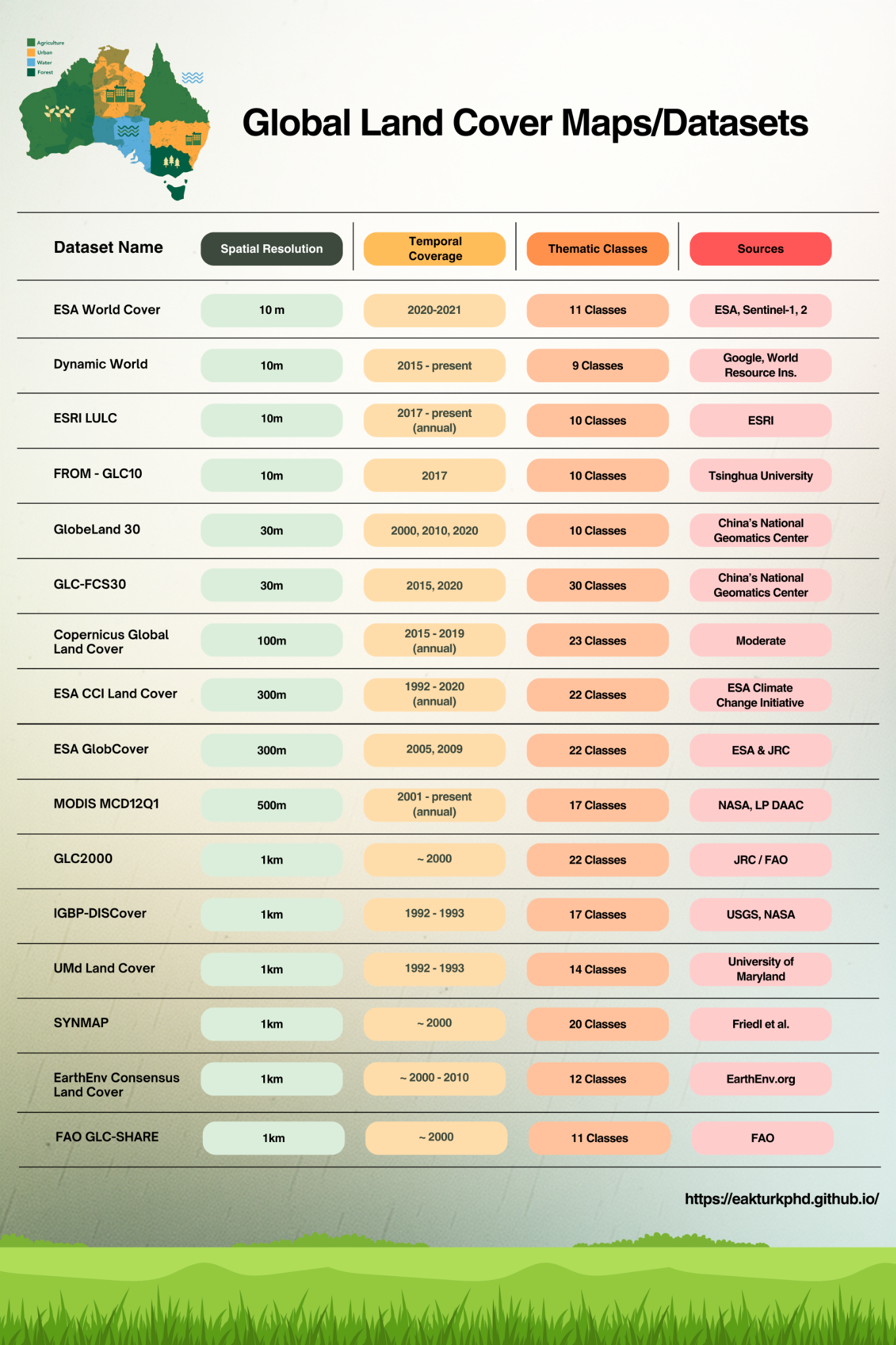
Main Global Land Cover Datasets
The summary figure below helps compare commonly used global land cover datasets in terms of resolution, temporal coverage, number of classes, and data provider. When reading the figure, three points deserve particular attention: which sensors were used to produce the dataset, which years it covers, and how closely its class definitions match the classes required for your study.
Five Critical Questions When Choosing a Dataset
When choosing a land cover dataset, the first feature considered is often spatial resolution. However, the decision process should not be reduced to the question of “10 m or 30 m?” The first critical question is the scale of the study. If small agricultural parcels, urban fringes, or narrow riparian zones are being examined, high-resolution products may offer an advantage. In contrast, if the focus is on continental-scale forest loss trends, drought pressure, or ecosystem modeling, coarser but more consistent time series may be preferable.
The second question is temporal coverage. A dataset may be very successful for a single reference year, but it may not be sufficient for long-term change analysis. The third question is whether the class scheme is suitable for the purpose of the study. For example, some datasets provide “forest” as a single category, while others offer subclasses such as closed forest, open forest, deciduous forest, or needle-leaved forest. This distinction directly affects the results, especially in forestry, carbon monitoring, and habitat suitability studies.
The fourth question concerns the sensor and production methodology. Optical data can be affected by cloud cover and atmospheric conditions, whereas radar data carry different types of information about structure, moisture, and surface roughness. For this reason, products that combine different data sources such as Sentinel-1 and Sentinel-2 may provide more stable results in certain geographies. The fifth, and perhaps most important, question is accuracy assessment. Even if the overall accuracy of a map appears high, user’s accuracy or producer’s accuracy may be low for specific classes. Therefore, rather than making decisions based on a single overall accuracy value, it is necessary to examine the class-level error structure.
The Most Common Mistake in Change Analysis
When working with land cover datasets, the most tempting but also the riskiest operation is to overlay two different years and produce a “change map.” At first glance, this approach seems straightforward: if a pixel was forest in 2015 and appears as cropland in 2020, then forest has converted to cropland. In practice, however, the situation is not always that simple. Classification errors, seasonal differences, cloud-mask problems, different sensor combinations, algorithm updates, and small changes in class definitions can blur the line between real change and mapping error.
Therefore, when conducting change analysis, the technical documentation of the dataset should be read, the same product family should be used whenever possible, classes should be simplified, and results should be supported with independent validation points. Especially when decisions will be made at the local scale, global land cover maps should usually be treated as starting data and evaluated together with field observations, high-resolution imagery, or national databases.
What Are These Datasets Used For?
The use of global land cover datasets is not limited to “producing maps.” Monitoring deforestation and reforestation processes, identifying agricultural expansion, modeling urban growth, tracking wetland losses, assessing post-fire landscape change, analyzing habitat fragmentation, and providing surface inputs for climate models are among their major applications.
These datasets also play an important role in monitoring indicators related to the Sustainable Development Goals. For example, land degradation neutrality, the protection of terrestrial ecosystems, water resource management, and climate adaptation policies cannot be evaluated properly without reliable land cover information. Therefore, land cover data are not merely technical products used by remote sensing experts; they are a common language for environmental management, planning, agriculture, forestry, disaster management, and climate policy.
Conclusion: Maps Tell Not Only the Surface, but Also the Story of Change
Global land cover datasets present the Earth’s surface to us as classified pixels. Yet what these pixels tell us is not merely “forest,” “cropland,” “water,” or “settlement.” Each pixel is a small part of a story where human activities and natural processes intersect. The contraction of a forest area in one place, the intensification of agriculture in another, the expansion of built-up areas along a coast, or the decline of a wetland are all spatial traces showing how the planet is changing.
For this reason, land cover datasets should not be seen merely as raster files to be downloaded, but as scientific infrastructures that make decision-making possible. When we match the right dataset with the right question, these maps do not only show the present; they also help us understand what has changed in the past and discuss more strongly what we need to protect in the future.
References
- FAO. (2020). Global Forest Resources Assessment 2020 – Main report. Food and Agriculture Organization of the United Nations.
- UNCCD. (2022). Desertification and Drought Day: Facts and figures (Land degradation statistics). United Nations Convention to Combat Desertification.
- Ramsar Convention on Wetlands. (2018). Global Wetland Outlook: State of the world’s wetlands and their services to people.
- Harrell, J. A., & Brown, V. M. (1992). The world’s oldest surviving geological map: The Turin Papyrus Map. Journal of Geology, 100(1), 3–18.
- Dilke, O. A. W. (1985). Greek and Roman Maps. Thames and Hudson.
- Kain, R. J. P., & Prince, H. C. (2000). Tithe Surveys of England and Wales. Cambridge University Press.
- USGS. (n.d.). Declassified satellite imagery (CORONA): Data access and overview. U.S. Geological Survey.
- USGS. (n.d.). Landsat 1 (ERTS-1) mission overview and history. U.S. Geological Survey.
- European Environment Agency. (n.d.). CORINE Land Cover: Background and programme history. EEA.
- USGS. (n.d.). National Land Cover Database (NLCD): Product suite and history. U.S. Geological Survey.
- Friedl, M. A., et al. (2010). MODIS Collection 5 global land cover: Algorithm refinements and characterization. Remote Sensing of Environment, 114(1), 168–182.
- Copernicus Land Monitoring Service. (n.d.). Service history and operational products. European Union / Copernicus.
- European Space Agency. (n.d.). ESA WorldCover: Worldwide land cover mapping and data access. ESA WorldCover.
- Brown, C. F., Brumby, S. P., Guzder-Williams, B., et al. (2022). Dynamic World, near real-time global 10 m land use land cover mapping. Scientific Data, 9, 251.
- Esri. (2024). Esri releases latest land cover map with updated Sentinel-2 satellite data. Esri Newsroom.
- Gong, P., Liu, H., Zhang, M., et al. (2019). Stable classification with limited sample: Transferring a 30-m resolution sample set collected in 2015 to mapping 10-m resolution global land cover in 2017. Science Bulletin, 64(6), 370–373.
- National Geomatics Center of China. (n.d.). GlobeLand30: 30-meter global land cover dataset.
- Zhang, X., Liu, L., Chen, X., Gao, Y., Xie, S., & Mi, J. (2021). GLC_FCS30: Global land-cover product with fine classification system at 30 m using time-series Landsat imagery. Earth System Science Data, 13, 2753–2776.
- Copernicus Land Monitoring Service. (n.d.). Land Cover 2015–2019 (raster 100 m), global, yearly – version 3. European Union / Copernicus.
- ESA Climate Change Initiative. (n.d.). Land Cover CCI product user guide and annual global land cover maps.
- NASA LP DAAC. (n.d.). MCD12Q1.061 MODIS Land Cover Type Yearly Global 500m. NASA Earthdata.